Multi-column statistics are back in SQL Server 2016

The new cardinality estimator in SQL Server 2014 brought new and improved query performance but as always there are caveats. Let’s check a specific case to see the different behaviors for the different versions of the CE Don’t get me wrong, they’ve always been there, but somehow someone forgot about them and weren’t used.

Since last week my mind has been on other things, I’m intending to write a series of articles and didn’t have much of my brain to get me write a post for this week, so finally I decided to speak about some issues which have been already described, but I believe they are good to be reminded.

 
What am I talking about? yeah, statistics

So statistics are the base for the cardinality estimator (CE from now on) to figure out how many rows will be returned by an operator during the execution of a query, I described some behaviors already in previous posts, so this time I’ll go a bit more to the specifics.

So far and for recent versions of SQL Server, we have 2 (I’d say 3) different versions of the CE. It was one of the big announcements for SQL Server 2014 and that left the picture like this.

• SQL Server 2012 and earlier version till 2000, CE version 70
• SQL Server 2014, new CE version 120

 
These numbers match with the compatibility level of the SQL Server versions they were released, coincidence? I don’t think so 🙂

So in SQL Server 2016 we have been given an improved version of the CE, which for the examples of this post, I think would be version 130.

I’m sure there are many small differences but I just want to talk about how the estimated number of rows differ from one version to another when we query a single table using two predicates and we have multi-column statistics that cover the combination.

In order to provide the 3 examples, I run my SQL Server 2016 Dev Edition instance with the sample database AdventureWorks2014.

Let’s get a fresh copy of the database and create the statistics

USE master
GO
IF DB_ID('AdventureWorks2014') IS NOT NULL BEGIN
	ALTER DATABASE AdventureWorks2014 SET SINGLE_USER WITH ROLLBACK IMMEDIATE
	DROP DATABASE AdventureWorks2014
END

RESTORE DATABASE AdventureWorks2014
FROM DISK = '.\AdventureWorks2014.bak'
WITH RECOVERY
, MOVE 'AdventureWorks2014_Data' TO 'C:\Program Files\Microsoft SQL Server\MSSQL13.MSSQL2016\MSSQL\DATA\AdventureWorks2014_Data.mdf'
, MOVE 'AdventureWorks2014_Log' TO 'C:\Program Files\Microsoft SQL Server\MSSQL13.MSSQL2016\MSSQL\DATA\AdventureWorks2014_Log.ldf'
GO

USE AdventureWorks2014

CREATE STATISTICS Person_Address_PostalCode_City ON Person.Address (PostalCode, City) WITH FULLSCAN

Once it’s done, we can test the different CE

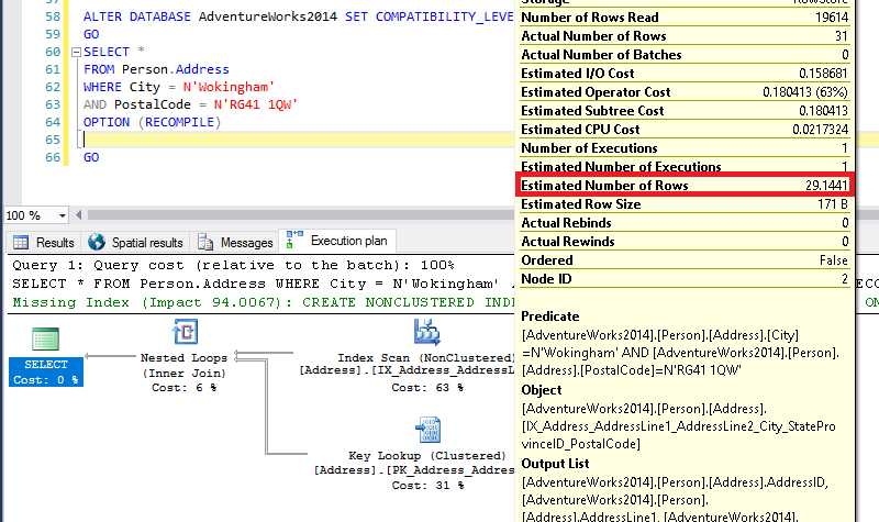
ALTER DATABASE AdventureWorks2014 SET COMPATIBILITY_LEVEL = 110 WITH ROLLBACK IMMEDIATE
GO
SELECT * 
FROM Person.Address
WHERE City = N'Wokingham'
AND PostalCode = N'RG41 1QW'
OPTION (RECOMPILE)
GO
-- 

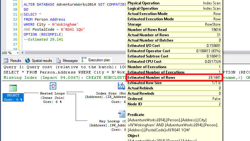
This estimated number comes from the statistics we have just created, if we have a look at them, I’ll show you the maths.

DBCC SHOW_STATISTICS ('Person.Address', 'Person_Address_PostalCode_City') 

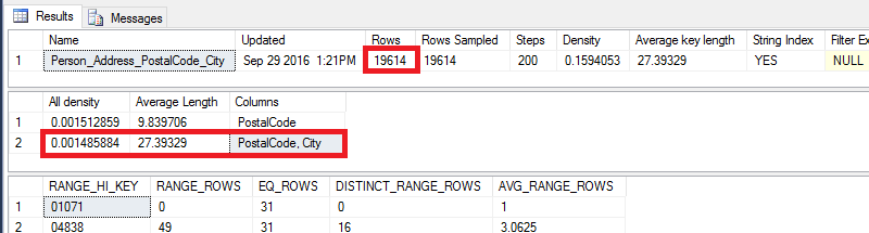
By multiplying the number of rows by the all density for the combination of columns, we get the number shown above 19614 * 0.001485884 = 29.144128776.

The actual rows is 31, so in this case the estimated are not far off the actual.

This is with the called ‘legacy CE’ so let’t see how is with the first review of the new CE

ALTER DATABASE AdventureWorks2014 SET COMPATIBILITY_LEVEL = 120 WITH ROLLBACK IMMEDIATE
GO
SELECT * 
FROM Person.Address
WHERE City = N'Wokingham'
AND PostalCode = N'RG41 1QW'
OPTION (RECOMPILE)
GO

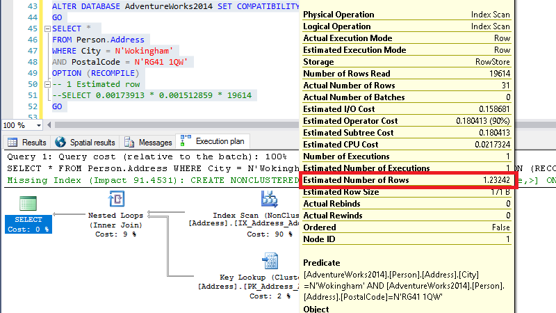
See how this is way off, all this marketing about the benefits of the new CE and this… Disappointing!

This version of the CE does not care about the existence of multi-column stats and just does the maths looking at single column stats.

If we look at the single column stats, we can work the numbers out

**Thanks to Fraser Watson for pointing this out

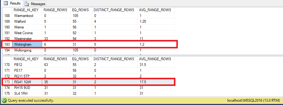
DBCC SHOW_STATISTICS ('Person.Address', 'City') WITH HISTOGRAM
DBCC SHOW_STATISTICS ('Person.Address', 'Person_Address_PostalCode_City') WITH HISTOGRAM

The new CE assumes some correlation between predicates within a single table, using the following formula

most selective * SQRT(2nd most selective) * number of rows

In our case the numbers are

SELECT  (CONVERT(FLOAT, 31) / 19614) * SQRT((CONVERT(FLOAT, 31) / 19614)) * 19614
-- 1.23242203675524

which makes the estimated value.

Forgetting about multi-column is bad in this case, probably it works better for some cases, but let’s see the facts

• ‘Wokingham’ has an estimate of 31 in the histogram of the column stats [City]
• ‘RG41 1QW’ has an estimate of 31 in the histogram of the multi column stats [Person_Address_PostalCode_City]

 
The average is 29 and the current is 31 just because both are directly correlated, but what if we were requesting a post code from a different city? The result would be zero, so 1,24 would be way better… Difficult to estimate correctly every time.

And finally, how things are in SQL Server 2016?

ALTER DATABASE AdventureWorks2014 SET COMPATIBILITY_LEVEL = 130 WITH ROLLBACK IMMEDIATE
GO
SELECT * 
FROM Person.Address
WHERE City = N'Wokingham'
AND PostalCode = N'RG41 1QW'
OPTION (RECOMPILE)
GO

Again we have the 29.1, so the new new CE is looking at multi column stats again.

 
Conclusion

The thing we can learn from this is that is impossible to be always right when you have to estimate the number of rows if your only resource is statistics, doesn’t matter single or multi-column, there is a set of values out there ready to defeat your logic.

However I think it’s a good idea that SQL Server 2016 gets back to look into multi-column for a simple reason, these are user created stats and therefore gives us (DBA’s, DEV’s) more power over how rows are estimated.

And With great power there must also come great responsibility, if we create multi-column stats randomly, we might be hurting performance for a lot of queries that would benefit from some correlation, but imagine we have for example dynamically loaded select lists which depend on the previous, this can be a great enhancement.

As always there’s no single truth. It will vary for each and every case, so test, test and test before opting for one or another.

Just to wrap up, a few links for reference.

• Statistics Used by the Query Optimizer in Microsoft SQL Server 2008 (White paper)
• Cardinality Estimator (SQL Server 2014)
• Cardinality Estimator (SQL Server 2016)
• Multi-column statistics and exponential backoff

 
Thanks for reading!