Fast with values slow with variables

There is a big debate why the same query can run fast with hard coded values and slow when using variables, come see there is a reasonable explanation for all this mess. The other day I saw a thread on linkedin groups that was titled ‘Using Parameters in a Query is Killing Performance’, where the author originally complaint because a query was running fine with hard coded values, but horribly slow when running with variables instead.

The variety of answers was big, giving all kind of recommendations always based on experience and best practices… hm mh

To find a proper explanation, let’s present a simple example where you can see by yourselves how the frustration the author is absolutely real.

I will use the [AdventureWorks2014] database to illustrate it, although since there are not so many rows in it, we must have a bit of imagination and extrapolate the results as if we were working with a bigger table.

First the query in two different versions, with the hard coded value and with then using an innocent variable to see why those are and behave differently

USE [AdventureWorks2014]

SELECT * 
	FROM Person.Address
	WHERE [StateProvinceID]  = 1
GO

USE [AdventureWorks2014]

DECLARE @StateProvince INT = 1

SELECT * 
	FROM Person.Address
	WHERE [StateProvinceID]  = @StateProvince
GO

As I told you earlier, this table has less than 20k rows, hence even the «horribly slow» version will be quite fast.

But, if we look at the query plans we can see they are very different, and that should be suspicious enough to investigate a bit more.

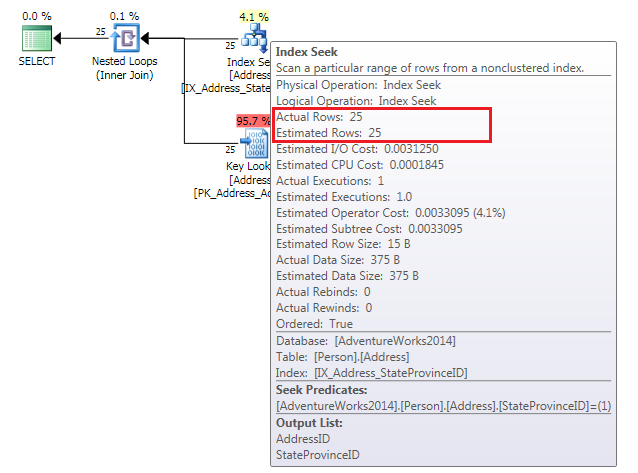
The first query’s execution plan shows an Index Seek to get the rows that match the condition (there is a non clustered index on this column) plus the Key Lookups to get the rest of the columns from the clustered index in this case.

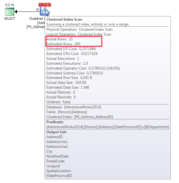
But the second one does not look quite the same, the optimizer in this case, has chosen a full Clustered Index Scan, see it there.

Why the second one has not done the same? If we compare the IO we can see the first one is far more efficient, achieving the result using less reads

/*
-- Index seek plus lookups
(25 row(s) affected)
Table 'Address'. Scan count 1, logical reads 52, physical reads 0, read-ahead reads 0, lob logical reads 0, lob physical reads 0, lob read-ahead reads 0.

(1 row(s) affected)


-- Clustered index scan
(25 row(s) affected)
Table 'Address'. Scan count 1, logical reads 346, physical reads 0, read-ahead reads 0, lob logical reads 0, lob physical reads 0, lob read-ahead reads 0.

(1 row(s) affected)

*/

Seven[~ish] times more reads using a full scan… the optimizer just gone crazy or what?

I want you to look at the Estimated Rows versus the Actual Rows, in the first query is the same but the second… Oh dear! more than 10 times bigger.

All this have an explanation (for sure), and we can see it if we look at the statistics for our non clustered index.

DBCC SHOW_STATISTICS ('[Person].[Address]', 'IX_Address_StateProvinceID')
GO

Which give us these numbers

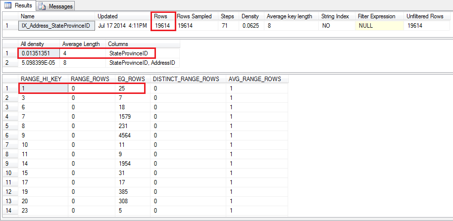
When looking at the histogram we can see that for [StateProvinceId] = 1 there are estimated 25 rows, nice! that is the right number.

This, though, does not explain why the second query estimate 265 rows for
[StateProvinceId] = @StateProvince

The thing is that when the query optimizer has to come up with a plan, is not aware of which value the variable will contain at the time of execution, hence it’s impossible to figure out what the [estimate] number of rows there will be, so it just take the average.

That is calculated multiplying the [Rows] from the first recordset 19614 by the [All Density] from the second recordset 0.01351351 = 265.05398514 and there you have your 265 estimated rows.

And what the optimizer knows for sure is for that many rows, the most optimal plan would be a Clustered Index Scan, you can prove it if you chose any province where the number of rows is close to 265 (see StateProvince 8, 19,20…). The plan generated for both is the same, Clustered Index Scan.

That’s why it’s so important not only to have accurate statistics, but knowing how SQL Server works internally to avoid unexpected surprises.

The ways to overcome this kind of situations is too long for this writing so I invite you to read about stats and query execution plans by yourselves.

Thanks for reading and please feel free to ask questions you may have.